Experimental part. A potential distribution in a thin conducting layer is used in this work as a two-dimensional model for an electrostatic field

A potential distribution in a thin conducting layer is used in this work as a two-dimensional model for an electrostatic field. To measure potential, a bridge is used (fig. 11.1). Two metal electrodes A and B are pressed to the sheet of paper with a conducting layer. Voltage U_o = 6.3 V passes from the source to electrodes and lower terminals of the potentiometer. Probe P is connected to the sliding contact S through terminals of vertical deflection of the oscilloscope (input Y).

The oscilloscope is used in the work as an indicator of presence of a potential difference. When the probe touches the surface of the conducting paper we observe a signal on oscilloscope screen (as a vertical intercept, height of which is proportional to a potential difference between a point of contact and sliding contact S). If potential at the point of contact is equal to one at sliding contact, a dot is seen on the screen.

Figure 11.1

At the beginning two or three sheets of paper with outlines of electrodes in the position taking place during the work have to be inserted under electrodes and conducting paper.

We consider potential of the electrode A to be equal to zero U_А = 0. Then U_В = 6.3 V (only an amplitude value of the potential is taken into account). To obtain an equipotential curve for some value , first it is needed to place sliding contact S in the appointed position (fig. 11.2)

. (11.6)

Then it is necessary to move probe P along the conducting layer in direction of decreasing oscilloscope signal and stop the probe when the signal becomes zero. Potential at the stop point is equal to U_i. In order to fix position of this point pierce all the sheets by top of the probe.

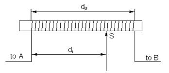
Figure 11.2

Near this point, another one with potential U_i has to be found and fixed. In such a way, moving from point to point, one can obtain the sequence of pinholes by which the equipotential curve can be drawn when the paper sheets are put out.

1. Obtain equipotential curves varying value of potential from 0 to 6.3 V with a step of 0.9 V. Take into consideration that outlines of electrodes are equipotential curves corresponding to potential values 0 and 6.3 V.

2. Build up a system of lines of force (not less than 7 in number).

3. Determine value and direction of an intensity at the points indicated by teacher. Value of intensity can be found by using the approximate formula

, (11.7)

where U_n and U_n+1 are potentials of two equipotential curves nearest to the point being considered; D is length of the shortest intercept joining these curves and coming through the point.

4. Estimate an error in location of equipotential curves

, (11.8)

where k (in V/a scale graduation) is position of the voltage divider at the Y input of the oscilloscope.