Main control laws

The control law or control algorithm is the algorithm used by the control processor to derive the actuator signal.

We introduce dimensionless relative variables:

where:

- some basic values (corresponding, say, to the nominal mode of an object).

1. Proportional law.

(2.9)

Such regulators are called proportional. Regulation process will be static.

is called a transfer coefficient of the regulator.

1. Integral law.

(2.10)

Constant has time dimension and is called the integration time constant.

1. Proportional plus integral law.

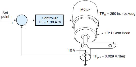
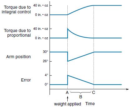
The introduction of integral control in a control system can reduce the steady-state error to zero. Integral control creates a restoring force that is proportional to the sum of all past errors multiplied by time.

For a constant value of error, the value of Σ(EΔt) will increase with time, causing the restoring force to get larger and larger. Eventually, the restoring force will get large enough to overcome friction and move the controlled variable in a direction to eliminate the error.

The system response of proportional + integral control

(2.11)

We may prove this ability of the mentioned regulator using this formula:

In the equilibrium state at constant input actions

it follows that the balance may be only at .

1. Proportional plus derivative law (PD law).

(2.12)

One solution to the overshoot problem is to include derivative control. Derivative control

“applies the brakes,” slowing the controlled variable just before it reaches its destination.

Mathematically, the contribution from derivative control is expressed in the following equation:

where

= controller output due to derivative control

= derivative gain constant (sometimes expressed , unit is time)

= proportional gain constant

= error rate of change (slope of error curve)

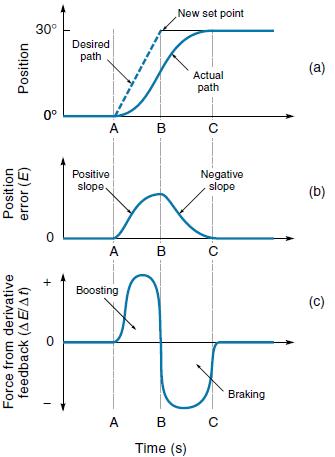
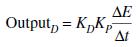
Figure above shows how a position control system with derivative feedback responds to a set-point change. Specifically, this Figure (a) shows the actual and desired position of the controlled variable, Figure (b) shows the position error (E), and Figure (c) shows the derivative control output.

Assume the controlled variable is initially at 0°. Then at time A the set point moves rapidly to 30°. Because of mechanical inertia, it takes time for the object to get up to speed. Notice that the

position error (E) is increasing (positive slope) during this time period (A to B).

Therefore, derivative control, which is proportional to error slope, will have a positive output, which gives the object a boost, to help get it moving. As the controlled variable closes in on the set-point value (B to C), the position error is decreasing (negative slope), so derivative feedback applies a negative force that acts like a brake, helping to slow the object.

For process control systems, where the set point is usually a fixed value, derivative control helps the system respond more quickly to load changes.