Classical theory of macroeconomic equilibrium. Partial, general and real equilibrium.

The key overall concepts in analyzing output, inflation, growth and the role of policy are aggregate demand and aggregate supply.

Aggregate demandis the relationship between spending on goods and services and the level of price. Aggregate demand curve tells us the quantity of goods and services people will buy for any given level of prices.

Aggregate demand curve shifts if non-price level determinants of aggregate demand changes (money supply, velocity of money, government spending and taxes, expectations and other factors).

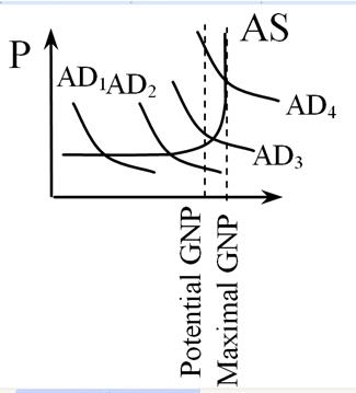
Aggregate supplygives a relationship between the general price level and the quantity of goods supplied. Non-price level determinants of aggregate supply are: changes in the size of the economy's labor force and its capital stock, productivity changes, changes in input prices, changes in taxes etc. All these changes shift the aggregate supply curve.

The relationship between the price level and the quantity of goods supplied depends crucially on the time horizon under consideration. We need to consider two cases: the long run, when all prices are flexible, and the short run, when some prices are sticky.

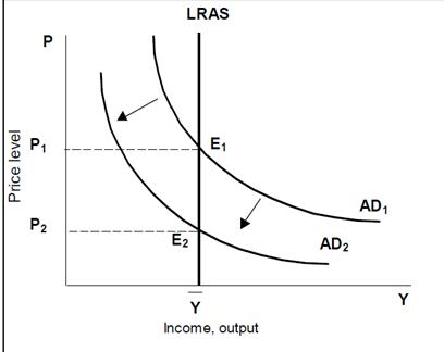
Since the classical modeldescribes how economy behaves in the long runwe derive the long run AS curve from the classical model. Classical economist supposed that market-oriented economy tended naturally to operate at a full-employment output level. They believed that prices and wages would always adjust quickly to clear markets and interest rate would always adjust to equate saving and investment. Changes in available stocks of capital or labour and technology improves shifts LRAS' curve.

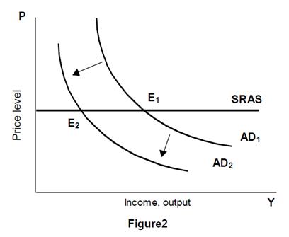
By contrast, the Keynesian modeldescribes short runfluctuations. Keynesian analysis focuses on how the equilibrium level of total income, output and employment is determined in an economy that operates at less than full employment and where the price level is not fully flexible.

Shifts in the AD curve, such as from AD1 to AD2 cause total output and employment to change (Figure 2). The equilibrium for the economy moves from point E1 to point E2 declining the total output (or sales), but not the price level as in the classical model.

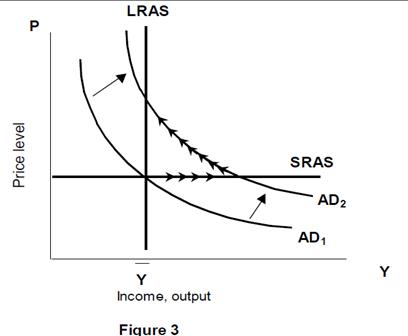
Now we need to explain how economy moves from short run equilibrium to the long run equilibrium. Suppose that economy begins in long run equilibrium (point A in Figure 3).

The Central Bank increases the money supply (we have positive aggregate demand curve shifts upward. In short run the increase in aggregate demand raises the output. At the old prices, firms sell more output. Economy moves from point A to point B (short run equilibrium), where output is above its natural-rate level (economic boom). Over time the high level of aggregate demand pulls up wages and prices. As the price level rises, the quantity of output demanded declines and the economy gradually moves downwards along the new aggregate demand curve AD2 to the point C, which is the new long-run equilibrium. In new equilibrium output and employment are back to their natural-rate levels, but prices are higher than in the old long-run equilibrium (point A).

2. Cyclical economic development. Characteristics phase’s cycle.